
一、神经网络算法:
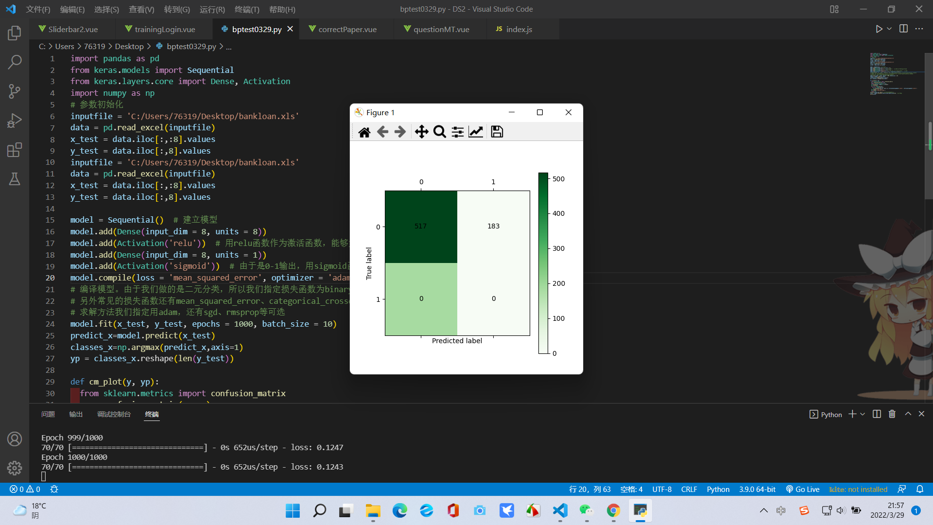
1import pandas as pd 2from keras.modelsimport Sequential 3from keras.layers.coreimport Dense, Activation 4import numpy as np 5# 参数初始化 6 inputfile ='C:/Users/76319/Desktop/bankloan.xls' 7 data = pd.read_excel(inputfile) 8 x_test = data.iloc[:,:8].values 9 y_test = data.iloc[:,8].values10 inputfile ='C:/Users/76319/Desktop/bankloan.xls'11 data = pd.read_excel(inputfile)12 x_test = data.iloc[:,:8].values13 y_test = data.iloc[:,8].values1415 model = Sequential()# 建立模型16 model.add(Dense(input_dim = 8, units = 8))17 model.add(Activation('relu'))# 用relu函数作为激活函数,能够大幅提供准确度18 model.add(Dense(input_dim = 8, units = 1))19 model.add(Activation('sigmoid'))# 由于是0-1输出,用sigmoid函数作为激活函数20 model.compile(loss ='mean_squared_error', optimizer ='adam')21# 编译模型。由于我们做的是二元分类,所以我们指定损失函数为binary_crossentropy,以及模式为binary22# 另外常见的损失函数还有mean_squared_error、categorical_crossentropy等,请阅读帮助文件。23# 求解方法我们指定用adam,还有sgd、rmsprop等可选24 model.fit(x_test, y_test, epochs = 1000, batch_size = 10)25 predict_x=model.predict(x_test)26 classes_x=np.argmax(predict_x,axis=1)27 yp = classes_x.reshape(len(y_test))2829def cm_plot(y, yp):30from sklearn.metricsimport confusion_matrix31 cm = confusion_matrix(y, yp)32import matplotlib.pyplot as plt33 plt.matshow(cm, cmap=plt.cm.Greens)34 plt.colorbar()35for xin range(len(cm)):36for yin range(len(cm)):37 plt.annotate(cm[x,y], xy=(x, y), horizontalalignment='center', verticalalignment='center')38 plt.ylabel('True label')39 plt.xlabel('Predicted label')40return plt41 cm_plot(y_test,yp).show()# 显示混淆矩阵可视化结果42 score = model.evaluate(x_test,y_test,batch_size=128)# 模型评估43print(score)
结果以及混淆矩阵可视化如下:
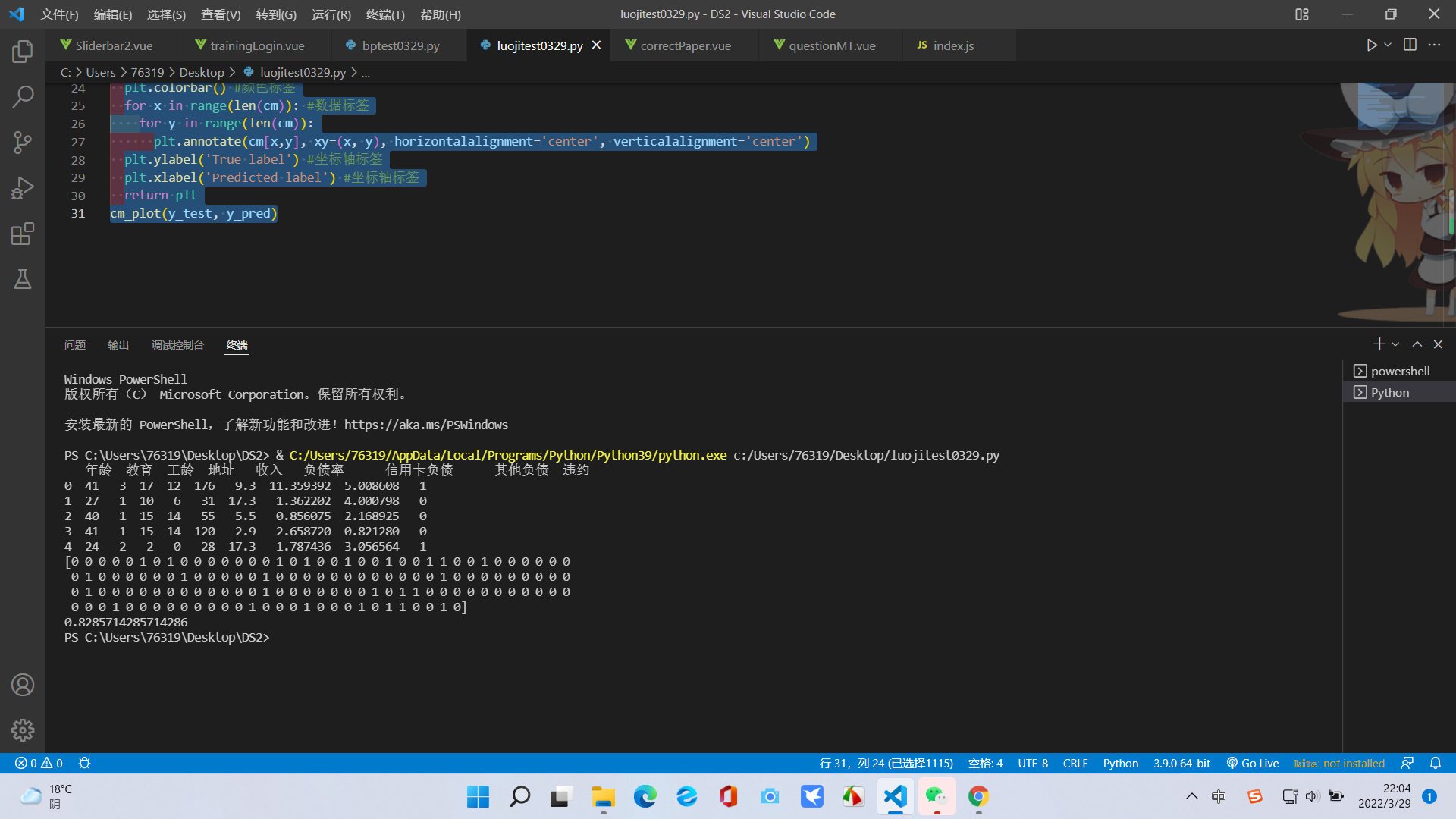
二、然后我们使用逻辑回归模型进行分析和预测:
import pandas as pd inputfile='C:/Users/76319/Desktop/bankloan.xls' data= pd.read_excel(inputfile)print (data.head()) X= data.drop(columns='违约') y= data['违约']from sklearn.model_selectionimport train_test_splitfrom sklearn.linear_modelimport LogisticRegression X_train, X_test, y_train, y_test= train_test_split(X, y, test_size=0.2, random_state=1) model= LogisticRegression() model.fit(X_train, y_train) y_pred= model.predict(X_test)print(y_pred)from sklearn.metricsimport accuracy_score score= accuracy_score(y_pred, y_test)print(score)def cm_plot(y, y_pred):from sklearn.metricsimport confusion_matrix#导入混淆矩阵函数 cm = confusion_matrix(y, y_pred)#混淆矩阵import matplotlib.pyplot as plt#导入作图库 plt.matshow(cm, cmap=plt.cm.Greens)#画混淆矩阵图,配色风格使用cm.Greens,更多风格请参考官网。 plt.colorbar()#颜色标签for xin range(len(cm)):#数据标签for yin range(len(cm)): plt.annotate(cm[x,y], xy=(x, y), horizontalalignment='center', verticalalignment='center') plt.ylabel('True label')#坐标轴标签 plt.xlabel('Predicted label')#坐标轴标签return plt cm_plot(y_test, y_pred).show()
结果如下:
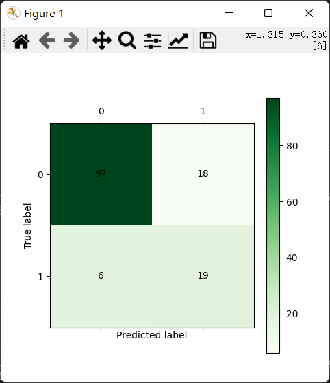
综上所述得出,两种算法模型总体上跑出来的准确率还是不错的,但是神经网络准确性更高一点。